
Creating a Time Series Table
Scenarios
Time series tables inherit the syntax of common column-store and row-store tables, making it easier to understand and use.
Time series tables can be managed through out data life cycle. Data increases explosively every day with a lot of dimensions. New partitions need to be added to the table periodically to store new data. Data generated a long time ago usually is of low value and is not frequently accessed. Therefore, it can be periodically deleted. Therefore, time series tables must have the capabilities of periodically adding and deleting partitions.
This practice demonstrates how to quickly create your time series tables and manage them by partitions. Specifying a proper type for a column helps improve the performance of operations such as import and query, making your service more efficient. The following figure uses genset data sampling as an example.
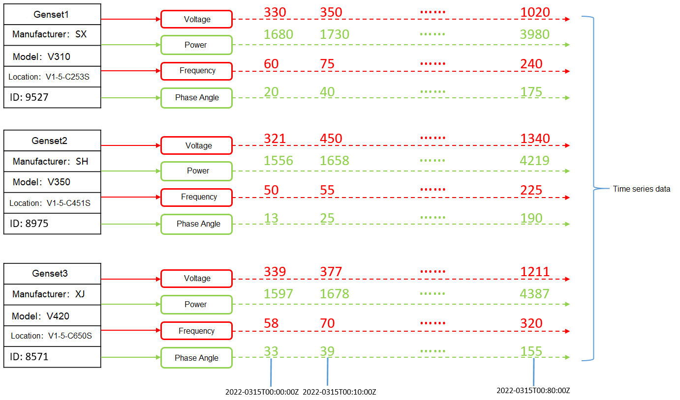

- The columns that describe generator attributes (generator information, manufacturer, model, location, and ID) are set as tag columns. During table creation, they are specified as TSTag
- The values of the sampling data metrics (voltage, power, frequency, and current phase angle) vary with time. During table creation, they are specified as TSField.
- The last column is specified as the time column, which stores the time information corresponding to the data in the field columns. During table creation, it is specified as TSTime.
Procedure
This practice takes about 30 minutes. The basic process is as follows:
Creating an ECS
For details, see Purchasing an ECS. After purchasing an ECS, log in to the ECS by referring to Logging In to a Linux ECS.

When creating an ECS, ensure that the ECS is in the same region, AZ, and VPC subnet as the stream data warehouse. Select the OS used by the gsql client (CentOS 7.6 is used as an example) as the ECS OS, and select using passwords to log in.
Creating a Stream Data Warehouse
- Log in to the Huawei Cloud management console.
- Choose Service List > Analytics > Data Warehouse Service. On the page that is displayed, click Create Cluster in the upper right corner.
- Configure the parameters according to Table 1.
Table 1 Software configuration Parameter
Configuration
Region
Select CN-Hong Kong.
NOTE:- CN-Hong Kong is used as an example. You can select other regions as required. Ensure that all operations are performed in the same region.
- Ensure that GaussDB(DWS) and the ECS are in the same region, AZ, and VPC subnet.
AZ
AZ2
Product
Stream data warehouse
Compute Resource
ECS
Storage Type
Cloud SSD
CPU Architecture
X86
Node Flavor
dwsx2.rt.2xlarge.m6 (8 vCPU | 64GB | 100-4,000 GB SSD)
NOTE:If this flavor is sold out, select other AZs or flavors.
Hot Storage
200 GB/node
Nodes
3
Cluster Name
dws-demo01
Administrator Account
dbadmin
Administrator Password
User-defined
Confirm Password
Enter the user-defined administrator password again.
Database Port
8000
VPC
vpc-default
Subnet
subnet-default(192.168.0.0/24)
NOTICE:Ensure that the cluster and the ECS are in the same VPC subnet.
Security Group
Automatic creation
EIP
Buy now
Enterprise Project
Default
Advanced settings
Default
- Confirm the information, click Next, and then click Submit.
- Wait for about 10 minutes. After the cluster is created, click the cluster name to go to the Basic Information page. Choose Network, click a security group name, and verify that a security group rule has been added. In this example, the client IP address is 192.168.0.x (the private network IP address of the ECS where gsql is located is 192.168.0.90). Therefore, you need to add a security group rule in which the IP address is 192.168.0.0/24 and port number is 8000.
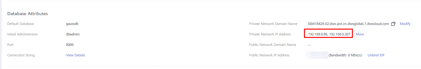
- Return to the Basic Information tab of the cluster and record the value of Private Network IP Address.
Using the gsql CLI Client to Connect to a Cluster
- Remotely log in to the Linux server where gsql is to be installed as user root, and run the following command in the Linux command window to download the gsql client:
1wget https://obs.ap-southeast-1.myhuaweicloud.com/dws/download/dws_client_8.1.x_redhat_x64.zip --no-check-certificate
- Decompress the client.
1cd <Path_for_storing_the_client> unzip dws_client_8.1.x_redhat_x64.zip
Where,
- <Path_for_storing_the_client>: Replace it with the actual path.
- dws_client_8.1.x_redhat_x64.zip: This is the client tool package name of RedHat x64. Replace it with the actual name.
- Configure the GaussDB(DWS) client.
1source gsql_env.sh
If the following information is displayed, the gsql client is successfully configured:
1All things done.
- Use the gsql client to connect to a GaussDB(DWS) database (using the password you defined when creating the cluster).
1gsql -d gaussdb -p 8000 -h 192.168.0.86 -U dbadmin -W password -r
If the following information is displayed, the connection succeeded:
1gaussdb=>
Creating a Time Series Table
- The following describes how to create a time series table GENERATOR for storing the sample data of gensets.
 1
 2
 3
 4
 5
 6
 7
 8
 9
10
11
CREATE TABLE IF NOT EXISTS GENERATOR(
genset text TSTag,
manufacturer text TSTag,
model text TSTag,
location text TSTag,
ID bigint TSTag,
voltage numeric TSField,
power bigint TSField,
frequency numeric TSField,
angle numeric TSField,
time timestamptz TSTime) with (orientation=TIMESERIES, period='1 hour', ttl='1 month') distribute by hash(model);
- Query the current time.
1
2
3
4
5
select now();
              now
-------------------------------
2022-05-25 15:28:38.520757+08
(1 row)
- Query the default partition and partition boundary.
1
2
3
4
5
6
7
8
9
SELECT relname, boundaries FROM pg_partition where parentid=(SELECT oid FROM pg_class where relname='generator') order by boundaries ;
    relname     |         boundaries
 ----------------+----------------------------
default_part_1 | {"2022-05-25 16:00:00+08"}
default_part_2 | {"2022-05-25 17:00:00+08"}
p1653505200    | {"2022-05-25 18:00:00+08"}
p1653541200    | {"2022-05-25 19:00:00+08"}
p1653577200    | {"2022-05-25 20:00:00+08"}
......
The TSTAG columns support the text, char, bool, int, and big int types.
The TSTime column supports the timestamp with time zone and timestamp without time zone types. It also supports the date type in databases compatible with the Oracle syntax. If time zone-related operations are involved, select a time type with time zone.
The data types supported by TSField columns are the same as those supported by column-store tables.

- To optimize the performance in time sequence scenarios, it is recommended to optimize the sequence of tag columns. To do so, prioritize writing more unique columns with distinct values at the beginning of table creation statements.
- When creating a time series table, set the table-level parameter orientation to timeseries.
- You do not need to manually specify DISTRIBUTE BY and PARTITION BY for a time series table. By default, data is distributed based on all tag columns, and the partition key is the TStime column.
- In the create table like syntax, the column names and the kv_type types are automatically inherited from the source table. If the source table is a non-time series table and the new table is a time series table, the kv_type type of the corresponding column cannot be determined. As a result, the creation fails.
- One and only one TSTIME attribute must be specified. Columns of the TSTIME type cannot be deleted. There must be at least one TSTag and TSField columns. Otherwise, an error will be reported during table creation.
Time series tables use the TSTIME column as the partition key and have the function of automatic partition management. Partition tables with the automatic partition management function help users greatly reduce O&M time. In the preceding table creation statement, you can see in the table-level parameters that two parameters period and ttl are specified for the time series table.
- period: interval for automatically creating partitions. The default value is 1 day. The value range is 1 hour ~ 100 years. By default, an auto-increment partition task is created for the time series table. The auto-increment partition task dynamically creates partitions to ensure that sufficient partitions are available for importing data.
- ttl: time for automatically eliminate partitions. The value range is 1 hour ~ 100 years. By default, no partition elimination task is created. You need to manually specify the partition elimination task when creating a table or use the ALTER TABLE syntax to set the partition elimination task after creating a table. The partition elimination policy is based on the condition that nowtime - partition boundary > ttl. Partitions that meet this condition will be eliminated. This feature helps users periodically delete obsolete data.
For partition boundaries
- If the period unit is hour, the start boundary value is the coming hour, and the partition interval is the value of period.
- If the period unit is day, the start boundary value is 00:00 of the coming day, and the partition interval is the value of period.
- If the period unit is month, the start boundary value is 00:00 of the coming month, and the partition interval is the value of period.
- If the period unit is year, the start boundary value is 00:00 of the next year, and the partition interval is the value of period.
Creating a Time Series Table (Manually Setting Partition Boundaries)
- Manually specify the start value of the partition boundary. For example, to manually set the default partition boundary time P1 to 2022-05-30 16:32:45 and P2 to 2022-05-31 16:56:12, and create a time series table GENERATOR1, run the following command:
 1
 2
 3
 4
 5
 6
 7
 8
 9
10
11
12
13
14
15
16
CREATE TABLE IF NOT EXISTS GENERATOR1(
genset text TSTag,
manufacturer text TSTag,
model text TSTag,
location text TSTag,
ID bigint TSTag,
voltage numeric TSField,
power bigint TSField,
frequency numeric TSField,
angle numeric TSField,
time timestamptz TSTime) with (orientation=TIMESERIES, period='1 day') distribute by hash(model)
partition by range(time)
(
PARTITION P1 VALUES LESS THAN('2022-05-30 16:32:45'),
PARTITION P2 VALUES LESS THAN('2022-05-31 16:56:12')
);
- Query the current time:
1
2
3
4
select now();
             now
-------------------------------
2022-05-31 20:36:09.700096+08(1 row)
- Run the following command to query partitions and partition boundaries:
1
2
3
4
5
6
7
8
SELECT relname, boundaries FROM pg_partition where parentid=(SELECT oid FROM pg_class where relname='generator1') order by boundaries ;
   relname   |         boundaries
-------------+----------------------------
p1          | {"2022-05-30 16:32:45+08"}
p2          | {"2022-05-31 16:56:12+08"}
p1654073772 | {"2022-06-01 16:56:12+08"}
p1654160172 | {"2022-06-02 16:56:12+08"}
......
Feedback
Was this page helpful?
Provide feedbackThank you very much for your feedback. We will continue working to improve the documentation.See the reply and handling status in My Cloud VOC.
For any further questions, feel free to contact us through the chatbot.
Chatbot


