Operator Basics

Operator Type

Type of an operator. For example, the type of a convolution operator is convolution. A network can have different operators of the same type.

Operator Name

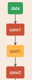
The name of an operator identifies the operator on a network. An operator name must be unique on a network. As shown in the following figure, conv1, pool1, and conv2 are the names of operators on the network. They are of the same type, convolution. Each indicates a convolution operation.

Figure 1 Network topology

Tensor

As data in a TE operator, the tensor includes the input data and output data. TensorDesc (the tensor descriptor) describes the input data and output data. Table 1 describes the attributes of the TensorDesc struct.

• Shape

  The shape of a tensor is described in the format of (D0, D1, ..., Dn – 1), where, D0 to Dn are positive integers.

  For example, the shape (3, 4) indicates a 3 x 4 matrix, where the first dimension has three elements, the second dimension has four elements.

  The number count in the bracket equals to the dimension count of the tensor. The first element of shape depends on the element count in the outer bracket of the tensor, and the second element of shape depends on the element count in the second bracket of the tensor starting from the left, and so on.

  Table 2 Tensor shape examples

  Tensor	Shape
  1	(0,)
  [1,2,3]	(3,)
  [[1,2],[3,4]]	(2,2)
  [[[1,2],[3,4]], [[5,6],[7,8]]]	(2,2,2)

• Format

  In the deep learning framework, n-dimensional data is stored by using an n-dimensional array. For example, a feature graph of a convolutional neural network is stored by using a four-dimensional array. The four dimensions are N, H, W and C, which stand for batch, height, width, and channels, respectively.

  Data can be stored only in linear mode because the dimensions have a fixed order. Different deep learning frameworks store feature graph data in different sequences. For example, data in Caffe is stored in the order of [Batch, Channels, Height, Width], that is, NCHW. Data in TensorFlow is stored in the order of [Batch, Height, Width, Channels], that is, NHWC.

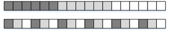
  As shown in Figure 2, an RGB picture is used as an example. In the NCHW order, the pixel values of each channel are clustered in sequence as RRRGGGBBB. In the NHWC order, the pixel values are interleaved as RGBRGBRGB.

  Figure 2 NCHW and NHWC
  

  To improve data access efficiency, the tensor data is in the Ascend AI software stack is stored in the 5D format NC1HWC0. C0 is closely related to the micro architecture and is equal to the size of the matrix computing unit in AI Core. For the FP16 type, C0 is 16; for the INT8 type, C0 is 32. The C0 data needs to be stored consecutively. That is, C1=(C+C0-1)/C0. If the division result is not an integer, the last data record is padded with zeros to be aligned with C0.

  The NHWC-to-NC1HWC0 conversion process is as follows:

  1. Split the NHWC data along dimension C into C1 pieces of NHWC0.
  2. Arrange the C1 pieces of NHWC0 in the memory consecutively into NC1HWC0.

Operator Attributes

Different operators have different attribute values. The following describes some common operator attributes.

• Axis

  The axis represents the subscript of a dimension of a tensor. For a two-dimensional tensor with five rows and six columns, that is, with shape (5, 6), axis 0 represents the first dimension in the tensor, that is, the row; axis 1 represents the second dimension of tensor, that is, the column.

  For example, for tensor [[[1,2],[3,4]], [[5,6],[7,8]]] with shape (2, 2, 2), axis 0 represents data in the first dimension, that is, matrices [[1,2],[3,4]] and [[5,6],[7,8]], axis 1 represents data in the second dimension, that is, arrays [1,2], [3,4], [5,6], and [7,8], and axis 2 indicates the data in the third dimension, that is, numbers 1, 2, 3, 4, 5, 6, 7, and 8.

  Negative axis is interpreted as a dimension counted from the end.

• Bias

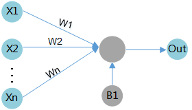
  The bias, along with the weight, is a linear component to be applied to the input data. It is applied to the result of multiplying the weight by the input data.

  As shown in Figure 3, assume that the input data is X1, the associated weight is W1, and the bias is B1. After the data passes the compute unit, the data changes to (X1 * W1 + B1).

  Figure 3 Bias computation example
  

• Weight

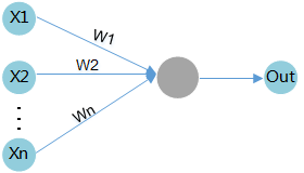
  The input data is multiplied by a weight value in the compute unit. For example, if an operator has two inputs, an associated weight value is allocated to each input. Generally, it is considered that relatively important data is assigned a relatively greater weight value, and a weight value of zero indicates a specific feature can be ignored.

  As shown in Figure 4, assume that the input data is X1 and the associated weight is W1. After the data passes the compute unit, the data changes to (X1 * W1).

  Figure 4 Weight computation example
  

Sample Operator: Reduction

Reduction is a Caffe operator that reduces the specified axis and its subsequent axes of a multi-dimensional array.

• Attributes of the reduction operator
  • ReductionOp: operation type. Four operation types are supported.

    Table 3 Operation types supported by the reduction operator

    Operator Type	Description
    SUM	Sums the values of all reduced axes.
    ASUM	Sums the absolute values of all reduced axes.
    SUMSQ	Squares the values of all reduced axes and then sums them.
    MEAN	Averages the values of all reduced axes.

  • axis: first axis to reduce. The value range is [–N, N – 1].
    For example, for an input tensor with shape (5, 6, 7, 8):

    • If axis = 3, the shape of the output tensor is (5, 6, 7).
    • If axis = 2, the shape of the output tensor is (5, 6).
    • If axis = 1, the shape of the output tensor is (5).
    • If axis = 0, the shape of the output tensor is (1).
  • coeff: scalar, scaling coefficient for output. The value 1 indicates that the output is not scaled.
• Data of the reduction operator
  • Input data

    The input contains the tensor data and tensor description.

    Input data: tensor x

    The description of tensor x contains the following attributes:

    Table 4 Input of the reduction operator

    Input Parameter	Description
    x	Name of the input tensor, whose shape is determined by the shape parameter
    shape	Shape of the input data, N-dimensional
    dtype	Type of the input data, either Indicates the data type. The value is float16 or float32.

  • Output data

    y: tensor of the identical data type as input x, whose shape is determined by the input tensor shape and the specified axis