Basic Concepts

RDD
Resilient Distributed Dataset (RDD) is a core concept of Spark. It indicates a read-only and partitionable distributed dataset. Partial or all data of this dataset can be cached in the memory and reused between computations.

RDD Generation
- An RDD can be generated from the Hadoop file system or other storage systems that are compatible with Hadoop, such as Hadoop Distributed File System (HDFS).
- A new RDD can be transferred from a parent RDD.
- An RDD can be converted from a collection.
RDD Storage
- Users can select different storage levels to store an RDD for reuse. (There are 11 storage levels to store an RDD.)
- The current RDD is stored in the memory by default. When the memory is insufficient, the RDD overflows to the disk.
RDD Dependency
The RDD dependency includes the narrow dependency and wide dependency.

Figure 1 RDD dependency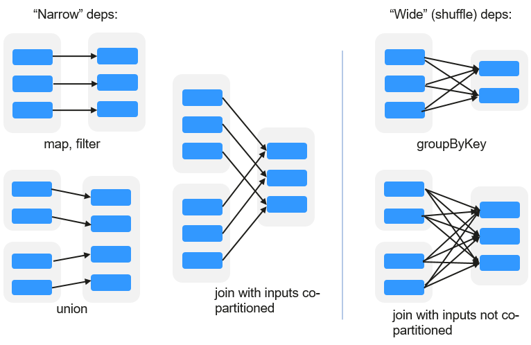
- Narrow dependency: Each partition of the parent RDD is used by at most one partition of the child RDD partition.
- Wide dependency: Partitions of the child RDD depend on all partitions of the parent RDD due to shuffle operations.
The narrow dependency facilitates the optimization. Logically, each RDD operator is a fork/join process. Fork the RDD to each partition, and then perform the computation. After the computation, join the results, and then perform the fork/join operation on next operator. It takes a long period of time to directly translate the RDD to physical implementation. There are two reasons: Each RDD (even the intermediate results) must be physicalized to the memory or storage, which takes time and space; the partitions can be joined only when the computation of all partitions is complete (if the computation of a partition is slow, the entire join process is slowed down). If the partitions of the child RDD narrowly depend on the partitions of the parent RDD, the two fork/join processes can be combined to optimize the entire process. If the relationship in the continuous operator sequence is narrow dependency, multiple fork/join processes can be combined to reduce the time for waiting and improve the performance. This is called pipeline optimization in Spark.
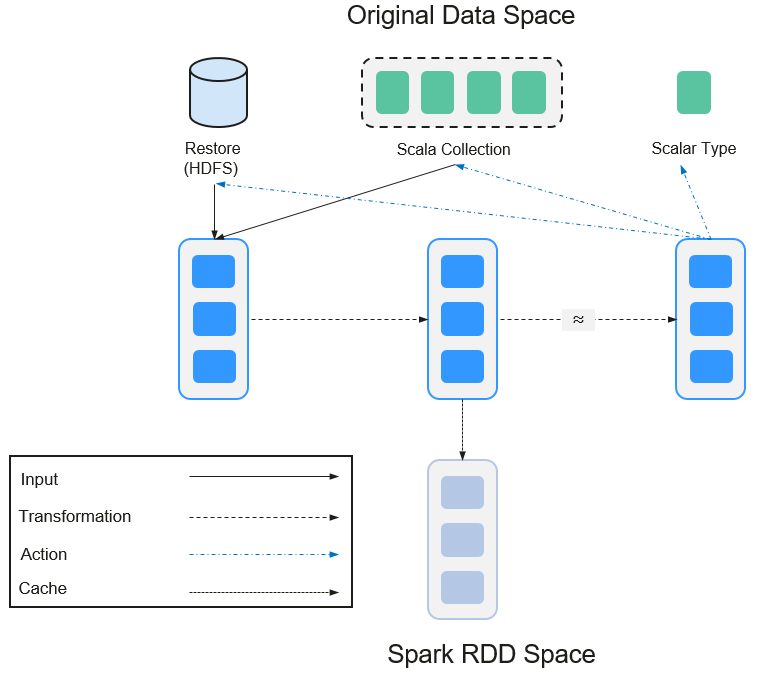
Transformation and Action (RDD Operations)
Operations on RDD include transformation (the returned value is an RDD) and action (the returned value is not an RDD). Figure 2 shows the process. The transformation is lazy, which indicates that the transformation from one RDD to another RDD is not immediately executed. Spark only records the transformation but does not execute it immediately. The real computation is started only when the action is started. The action returns results or writes the RDD data into the storage system. The action is the driving force for Spark to start the computation.

Figure 2 RDD operation

The data and operation model of RDD are quite different from those of Scala.
```
val file = sc.textFile("hdfs://...") val errors = file.filter(_.contains("ERROR")) errors.cache() errors.count()
```
1. The textFile operator reads log files from the HDFS and returns file (as an RDD).
2. The filter operator filters rows with ERROR and assigns them to errors (a new RDD). The filter operator is a transformation.
3. The cache operator caches errors for future use.
4. The count operator returns the number of rows of errors. The count operator is an action.
Transformation includes the following types:
- The RDD elements are regarded as simple elements:
  The input and output have the one-to-one relationship, and the partition structure of the result RDD remains unchanged, for example, map.
  
  The input and output have the one-to-many relationship, and the partition structure of the result RDD remains unchanged, for example, flatMap (one element becomes a sequence containing multiple elements and then flattens to multiple elements).
  
  The input and output have the one-to-one relationship, but the partition structure of the result RDD changes, for example, union (two RDDs integrates to one RDD, and the number of partitions becomes the sum of the number of partitions of two RDDs) and coalesce (partitions are reduced).
  
  Operators of some elements are selected from the input, such as filter, distinct (duplicate elements are deleted), subtract (elements only exist in this RDD are retained), and sample (samples are taken).
- The RDD elements are regarded as Key-Value pairs.
  Perform the one-to-one calculation on the single RDD, such as mapValues (the partition mode of the source RDD is retained, which is different from map).
  
  Sort the single RDD, such as sort and partitionBy (partitioning with consistency, which is important to the local optimization).
  
  Restructure and reduce the single RDD based on key, such as groupByKey and reduceByKey.
  
  Join and restructure two RDDs based on key, such as join and cogroup.
  
  The later three operations involve sorting and are called shuffle operations.
Action is classified into the following types:
- Generate scalar configuration items, such as count (the number of elements in the returned RDD), reduce, fold/aggregate (the number of scalar configuration items that are returned), and take (the number of elements before the return).
- Generate the Scala collection, such as collect (import all elements in the RDD to the Scala collection) and lookup (look up all values corresponds to the key).
- Write data to the storage, such as saveAsTextFile (which corresponds to the preceding textFile).
- Check points, such as checkpoint. When Lineage is quite long (which occurs frequently in graphics computation), it takes a long period of time to execute the whole sequence again when a fault occurs. In this case, checkpoint is used as the check point to write the current data to stable storage.
Shuffle
Shuffle is a specific phase in the MapReduce framework, which is located between the Map phase and the Reduce phase. If the output results of Map are to be used by Reduce, each output result must be hashed based on the key and distributed to the corresponding Reducer. This process is called Shuffle. Shuffle involves the read and write of the disk and the transmission of the network, so that the performance of Shuffle directly affects the operation efficiency of the entire program.

The following figure describes the entire process of the MapReduce algorithm.

Figure 3 Algorithm process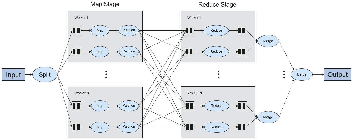

Shuffle is a bridge connecting data. The following describes the implementation of shuffle in Spark.

Shuffle divides the Job of a Spark into multiple stages. The former stages contain one or multiple ShuffleMapTasks, and the last stage contains one or multiple ResultTasks.
Spark Application Structure
The Spark application structure includes the initial SparkContext and the main program.
- Initial SparkContext: constructs the operation environment of the Spark application.
  Constructs the SparkContext object. Example:,
```
new SparkContext(master, appName, [SparkHome], [jars])
```
  Parameter description
  
  master: indicates the link string. The link modes include local, YARN-cluster, and YARN-client.
  
  appName: indicates the application name.
  
  SparkHome: indicates the directory where Spark is installed in the cluster.
  
  jars: indicates the code and dependency package of the application.
- Main program: processes data.
For submitting applications details, see https://spark.apache.org/docs/3.1.1/submitting-applications.html
Spark shell Command
The basic Spark shell command supports the submitting of the Spark application. The Spark shell command is
```
./bin/spark-submit \
 --class <main-class> \
 --master <master-url> \ 
... # other options 
 <application-jar> \ 
 [application-arguments]
```
Parameter description:

--class: indicates the name of the class of the Spark application.

--master: indicates the master that the Spark application links, such as YARN-client and YARN-cluster.

application-jar: indicates the path of the jar package of the Spark application.

application-arguments: indicates the parameter required to submit the Spark application. (This parameter can be empty.)
Spark JobHistory Server
The Spark Web UI is used to monitor the details in each phase of the Spark framework of a running or historical Spark job and provide the log display, which helps users to develop, configure, and optimize the job in more fine-grained units.

Spark SQL Basic Concepts

DataSet

A DataSet is a strongly typed collection of domain-specific objects that can be transformed in parallel using functional or relational operations. Each Dataset also has an untyped view called a DataFrame, which is a Dataset of Row.

DataFrame is a structured distributed data set composed of several columns, which is similar to a table in the relationship database or the data frame in R/Python. DataFrame is a basic concept in Spark SQL, and can be created by using multiple methods, such as structured data set, Hive table, external database, or RDD.

Spark Streaming Basic Concepts

Dstream

The DStream (Discretized Stream) is an abstract concept provided by the Spark Streaming.

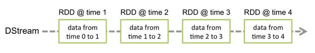
The DStream is a continuous data stream which is obtained from the data source or transformed and generated by the inflow. In essence, a DStream is a series of continuous RDDs. The RDD is a distributed dataset which can be read only and divided into partitions.

Each RDD in the DStream contains the data of a partition as shown in Figure 4.

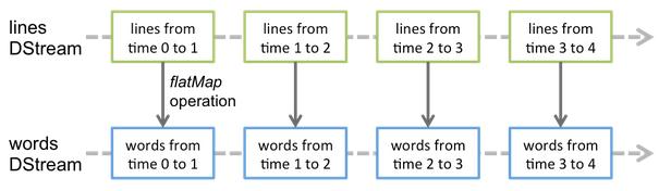
Figure 4 Relationship between DStream and RDD

All operators applied in the DStream are translated to the operations in the lower RDD as shown in Figure 5. The transformation of the lower RDDs is calculated by using the Spark engine. Most operation details are concealed in the DStream operators and High-level APIs are provided for developers.

Figure 5 DStream operator transfer

Structured Streaming Basic Concepts

Input Source
Input data sources. Data sources must support data replay based on the offset. Different data sources have different fault tolerance capabilities.
Sink
Data output. Sink must support idempotence write operations. Different Sinks have different fault tolerance capabilities.
outputMode
Result output mode, which can be:
- Complete Mode: The entire updated result table will be written to the external storage. It is up to the storage connector to decide how to handle writing of the entire table.
- Append Mode: If an interval is triggered, only the new rows appended in the Result Table will be written into an external system. This mode is applicable only to a result set that has already existed and will not be updated.
- Update Mode: If an interval is triggered, only updated data in the Result Table will be written into an external system, which is a difference between the Appendix Mode and Update Mode.
Trigger
Output trigger. Currently, the following trigger types are supported:
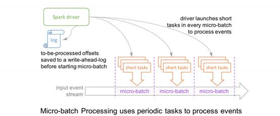
- Default: Micro-batch mode. After a batch is complete, the next batch is automatically executed.
- Specific interval: Processing is performed at a specific interval.
- One-time execution: Query is performed only once.
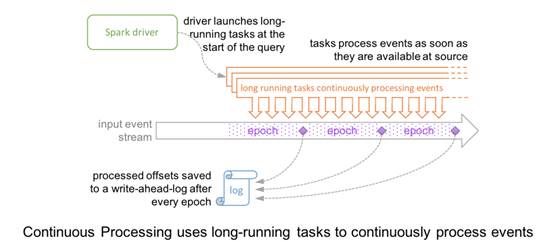
- Continuous mode: This is an experimental feature. In this mode, the stream processing delay can be decreased to 1 ms.

Structured Streaming supports the micro-batch mode and continuous mode. The micro-batch mode cannot ensure low-delay but has a larger throughput within the same time. The continuous mode is suitable for data processing requiring millisecond-level delay, which is an experimental feature.

In the current version, if the stream-to-batch joins function is required, outputMode must be set to Append Mode.

Figure 6 Running process in micro-batch mode